
PROJECT CONTROLS GUIDE
How to Analyze Project Cost Variances
Analyzing project cost variances requires more than comparing actual costs with the approved budget. This guide provides a practical approach to establish reliable cost baselines, measure cost performance, identify significant variances, investigate root causes, forecast final costs, take corrective action, monitor results, and strengthen cost control throughout project delivery.
Practical Guide · Project Controls
The Project Cost Variance Analysis Challenge
A cost variance does not explain the problem
Consider a project reporting:Actual Cost: $52 million | Budget: $48 million | Variance: $4 million unfavourableThe figures identify a financial deviation. However, they do not tell management which cost elements created the variance, when the problem began, or whether the exposure will continue. The team therefore needs to move beyond the number and investigate the underlying conditions.
Cost overruns remain a persistent industry problem
Research across construction and infrastructure projects continues to identify cost overruns as a significant project-management challenge. A 2024 systematic review of construction cost-control practices identified techniques such as variance analysis, budget monitoring, resource monitoring, interim valuation, and unit costing as important approaches to cost control. Similarly, research reviewing more than 300 publications identified 73 studies addressing time and cost overruns in construction projects. These findings show why project teams need active cost control throughout execution rather than relying only on the original estimate.One variance can have several connected causes
A cost variance may appear in one cost account while its underlying cause exists somewhere else. For example:Higher installation cost → Low productivity → Material availability problems → Procurement delay → Late engineering releaseThe additional installation cost may therefore represent a consequence rather than the root cause. Furthermore, scope changes, quantity growth, price escalation, productivity losses, rework, procurement problems, schedule delays, risks, and commercial issues can interact. Consequently, effective Project Cost Variances analysis requires the team to examine relationships across cost, schedule, progress, procurement, resources, risk, and change.
Poor data can weaken the analysis
Reliable analysis depends on reliable information. Project teams may need to reconcile budgets, actual costs, commitments, accruals, earned value, progress, changes, procurement information, and resource costs. However, different functions may use different reporting dates, coding structures, assumptions, or levels of detail. As a result, teams can spend significant effort reconciling information before they can explain the variance. Therefore, cost variance analysis starts with consistent and validated project information.Current cost performance does not guarantee the final outcome
A project can show an acceptable current cost position while its final exposure continues to increase. Outstanding commitments, unfinished high-cost work, unresolved risks, declining productivity, pending changes, and schedule pressure can all affect the remaining cost. Consequently, the current variance cannot provide the complete financial outlook. The team must also consider remaining work, commitments, risks, productivity, corrective actions, and the estimate at completion.The real challenge is turning variance into action
Ultimately, project teams do not analyze cost variances simply to produce another monthly report. They need the analysis to answer:What changed? Why did it change? What will it mean for the final cost? What should we do now?Therefore, effective cost variance analysis must connect measurement, root-cause analysis, forecasting, corrective action, monitoring, and learning. That distinction sets the foundation for the next section of this guide: understanding why project cost variances occur and why teams often struggle to identify their underlying causes.
Why Project Cost Variances Are Difficult to Analyze
Accurate project cost variance analysis rarely fails because teams lack financial data. More often, the problem comes from how teams establish the cost baseline, measure performance, classify costs, connect financial information with project progress, and interpret the reasons behind variances.
The following causes highlight the major weaknesses that can make cost variance analysis misleading, incomplete, or difficult to act upon.
1. Inaccurate or Unrealistic Cost Estimates
Cost variance problems can begin before project execution when the estimate does not reflect realistic delivery conditions.
For example, teams may use optimistic productivity rates, incomplete quantities, outdated market prices, limited historical data, or insufficient allowances for uncertainty.
As a result, the approved cost baseline may already contain assumptions that the project cannot realistically achieve.
Therefore, when actual costs exceed the baseline, the team needs to determine whether the variance reflects poor execution, unrealistic assumptions, or both.
Without this distinction, management may focus on correcting project performance while the underlying estimating weakness remains unresolved.
2. Unclear Scope and Changing Requirements
Project costs can change significantly when the scope continues to evolve after the team establishes the baseline.
Design development, changing requirements, additional deliverables, quantity growth, and scope creep can increase labour, material, procurement, and subcontract costs.
However, not every cost increase represents poor cost control.
Some increases may result from approved changes, while others may originate from inadequate scope definition or uncontrolled requirements.
Therefore, the project team needs to distinguish approved scope growth, emerging changes, and genuine cost-performance problems before interpreting the variance and deciding what corrective action the project requires.
3. Low Productivity and Execution Inefficiency
A project can spend more than planned because the team produces less work for the resources consumed.
Low labour productivity, inefficient equipment utilization, rework, poor sequencing, site constraints, and unexpected work complexity can all increase the cost of completed work.
However, the cost report alone may not reveal these operational conditions.
Therefore, the project controls team should connect cost performance with physical progress, completed quantities, labour hours, equipment usage, and productivity trends.
This approach helps the team determine whether additional expenditure reflects genuine progress or whether inefficient execution is driving the unfavorable cost variance.
4. Weak Progress Measurement Distorts Cost Performance
A project can spend more than planned because the team produces less work for the resources consumed.
Low labour productivity, inefficient equipment utilization, rework, poor sequencing, site constraints, and unexpected work complexity can all increase the cost of completed work.
However, the cost report alone may not reveal these operational conditions.
Therefore, the project controls team should connect cost performance with physical progress, completed quantities, labour hours, equipment usage, and productivity trends.
This approach helps the team determine whether additional expenditure reflects genuine progress or whether inefficient execution is driving the unfavorable cost variance.
5. Poor Cost and Project Data Quality
Project cost analysis often combines information from finance, procurement, planning, commercial teams, contractors, and other functions.
However, these sources may use different reporting dates, cost codes, assumptions, or levels of detail.
As a result, the project team may spend considerable time reconciling information before it can understand the actual variance.
Missing commitments, delayed accruals, incorrect coding, or incomplete actual costs can further distort the reported position.
Therefore, effective analysis requires timely, consistent, validated, and traceable project cost information before management can rely on the results and make informed decisions.
6. Schedule Delays Create Additional Cost Exposure
Schedule delays can create additional costs even when the project team does not directly increase the planned scope.
Extended labour, equipment usage, supervision, site overheads, temporary facilities, and subcontractor costs can increase as the project duration extends.
Therefore, a cost variance may originate from a schedule problem rather than from direct overspending within the affected cost account.
The team should consequently examine schedule trends, critical activities, remaining duration, and productivity alongside cost performance.
This integrated approach helps the team understand whether schedule deterioration is creating additional cost exposure and whether management needs to intervene before the impact increases.
7. Procurement and Market Conditions Change the Cost Position
Market conditions can change the project’s expected cost after the team establishes the baseline.
Material prices, labour rates, exchange rates, inflation, supplier conditions, and availability can all influence procurement costs.
At the same time, procurement delays can expose the project to price increases, expedited transportation, alternative sourcing, or contractual consequences.
Therefore, the team needs to distinguish market-driven cost exposure from controllable execution performance.
This distinction matters because each situation requires a different response. Procurement intervention, commercial action, risk treatment, or operational improvement may be appropriate depending on the actual cause.
8. Variances Often Show Symptoms Rather Than Root Causes
A cost variance identifies a difference from the approved cost reference, but it does not automatically explain its cause.
The visible variance may represent a symptom of a problem that originated in another project function.
For example, higher installation costs may result from low productivity, while low productivity may result from material shortages caused by procurement delays.
Therefore, the team needs to investigate beyond the affected cost account and distinguish direct causes, contributing factors, and underlying causes.
Without this deeper analysis, corrective action may address the visible symptom while the actual problem continues to affect project cost.
9. Forecasts Can Remain Too Optimistic
A project can continue reporting an optimistic final cost forecast even after unfavorable performance becomes visible.
Teams may assume that future productivity will improve, remaining work will proceed according to plan, or identified risks will not materialize.
However, these assumptions can delay recognition of the project’s actual financial exposure.
Therefore, the team should challenge the forecast using current productivity, remaining work, commitments, risks, changes, and historical performance.
A credible estimate at completion should reflect evidence from current project conditions rather than simply repeat the original budget or assume that previous cost problems will automatically disappear.
10. Organizational Pressure Can Delay Recognition
Cost variance analysis also depends on the project’s reporting culture.
Teams may hesitate to report unfavorable performance because they expect blame, stakeholder resistance, commercial consequences, or pressure to maintain an approved forecast.
Consequently, a project can have technically capable controls but still recognize problems too late.
Management should therefore encourage transparent reporting, evidence-based challenge, clear accountability, and early escalation.
When teams can report unfavorable information openly, project leaders gain more time to investigate causes, evaluate recovery options, and take corrective action before the financial exposure becomes more difficult to manage.
11. Poorly Structured Control Accounts Hide Cost Drivers
The structure used to organize project costs affects how easily the team can explain a variance.
If a control account combines unrelated work, resources, materials, subcontractors, or activities, one unfavorable result may contain several different cost drivers.
Consequently, management may see the total variance without understanding which component requires attention.
The project should therefore establish control accounts and cost structures at a useful level of detail.
The structure should provide enough visibility to identify meaningful cost drivers while avoiding excessive administrative effort, unnecessary reporting complexity, and excessive fragmentation of project information.
12. Weak Link Between Variance Analysis and Corrective Action
Identifying and explaining a cost variance does not automatically improve project performance.
Some teams report the variance, document a general explanation, and repeat the same information during the next reporting cycle without addressing the underlying problem.
Effective project controls should instead connect variance → cause → impact → forecast → action → follow-up.
Each significant variance should lead to an appropriate response with a clear owner, target date, expected outcome, and follow-up measure.
Otherwise, cost variance analysis becomes a reporting activity rather than an active mechanism for controlling project performance and improving the final outcome.
What Should You Do?
Effective cost variance analysis requires more than identifying whether actual costs differ from the budget. The project team needs a structured approach that connects baseline, actual cost, progress, variance, root cause, forecast, and corrective action.
The following seven steps provide a practical control cycle that helps teams understand cost performance, identify emerging problems, and take timely action based on reliable project evidence.
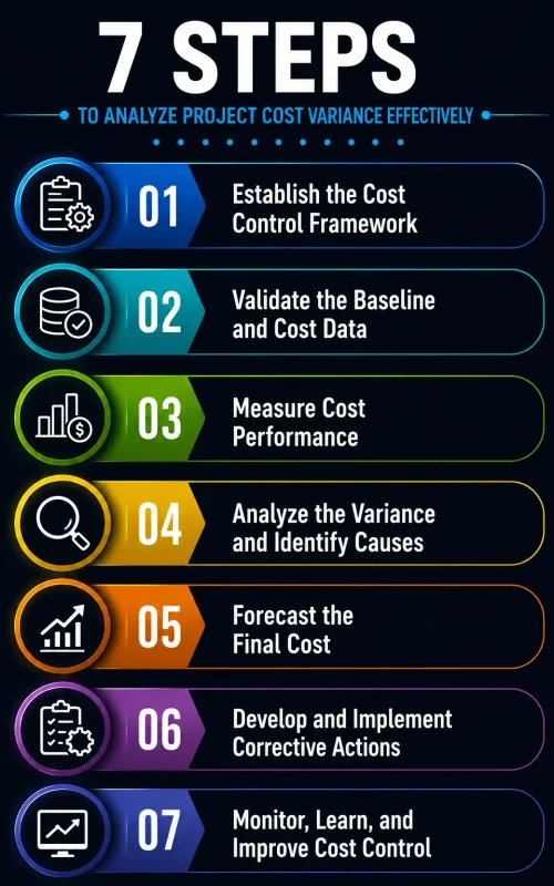
Step 1 — Establish a Reliable Cost Baseline
Before analyzing project cost variances, the team needs a reliable reference point. Without an approved and properly structured cost baseline, the comparison between planned and actual costs can produce misleading results.
The objective is not simply to create a budget. Instead, the team needs to establish a controlled cost baseline that reflects the approved scope, planned execution strategy, schedule, resources, and known project assumptions.
Define the approved project scope
Start by confirming exactly what the project budget covers. Review the approved scope, work breakdown structure, contract requirements, deliverables, and major work packages.
This step helps prevent the team from comparing actual costs against a budget that excludes important work or includes costs outside the approved project scope.
Structure the cost baseline
Organize the approved budget into a structure that allows the team to identify meaningful cost variances.
Depending on the project, the structure may include:
- Work packages and control accounts
- Labour and equipment
- Materials and procurement
- Subcontracts
- Engineering and other project services
- Indirect and project overhead costs
The structure should provide enough detail to identify cost drivers without creating unnecessary administrative complexity.
Align cost with schedule and scope
Cost information becomes more useful when the team can connect it with planned work and project timing.
Therefore, align the cost baseline with the work breakdown structure, schedule, control accounts, and planned time-phasing wherever appropriate.
This alignment allows the team to understand not only how much the project planned to spend, but also when and on which work the project expected to incur that cost.
Document baseline assumptions
Record the assumptions that support the approved budget. These may include productivity rates, material prices, labour rates, quantities, exchange rates, procurement conditions, resource requirements, and planned execution methods.
These assumptions provide important context when the team later investigates a cost variance. They also help distinguish baseline assumption changes from genuine cost-performance problems.
Control baseline changes
Finally, establish a formal process for approving and recording changes to the cost baseline.
Do not overwrite the original baseline simply because project conditions change. Instead, maintain appropriate records of approved changes so the team can understand the original plan, current approved position, and reasons for movement.
Key outcome: At the end of Step 1, the project should have a clear, approved, time-phased, and traceable cost baseline that provides a credible foundation for analyzing project cost variances.
Step 2 — Collect and Validate Actual Cost Information
Once the cost baseline is established, the next step is to build a reliable picture of the costs the project has actually incurred and committed.
Cost variance analysis becomes unreliable when actual costs arrive late, remain incomplete, use inconsistent classifications, or do not align with the approved cost structure. Therefore, the team should establish a consistent process for collecting, validating, reconciling, and reporting actual cost information before calculating significant variances.
Define the actual cost data requirements
First, identify the information required to understand the project’s current cost position. Depending on the project, this may include:
- Actual costs incurred
- Committed costs
- Accruals for work completed but not yet invoiced
- Labour and equipment costs
- Material and procurement costs
- Subcontractor costs
- Indirect and project overheads
- Approved changes
Define these requirements before each reporting cycle so that different functions provide information consistently.
Align actual costs with the cost structure
Actual costs should follow the same cost structure used for the baseline wherever practical.
For example, if the baseline separates engineering, procurement, construction, and commissioning costs, actual expenditure should allow the team to identify costs against those same areas.
This alignment makes it easier to determine where the variance occurred, which work generated it, and which cost drivers require investigation.
Capture commitments and accruals
Actual expenditure alone may not represent the project’s current financial exposure.
Committed costs can include purchase orders, subcontract commitments, and other obligations that the project has already created. Similarly, accruals can capture costs associated with work already performed but not yet recorded through invoices.
Therefore, review actuals, commitments, and relevant accruals together when assessing the current cost position.
Validate the information
Before using the data for variance analysis, perform basic quality checks.
- Check whether all required cost information has arrived.
- Confirm that costs use the correct cost codes.
- Review unusual increases or decreases.
- Check whether accruals reflect actual work performed.
- Confirm that major commitments appear in the records.
- Investigate missing or duplicated transactions.
These checks help prevent data-quality problems from becoming misleading cost variances.
Reconcile information across functions
Cost information should also agree with the wider project position.
For example, significant procurement costs should correspond with procurement activity, while subcontract costs should reasonably reflect the work performed and contractual position.
Similarly, cost information should align with the project status date and reporting period. This reconciliation provides an additional check before the team interprets the variance.
Key outcome: At the end of Step 2, the project should have complete, timely, validated, and consistently classified actual cost information that can be reliably compared with the approved baseline.
Step 3 — Measure Earned Value and Identify Cost Variances
After collecting and validating actual cost information, the project team needs to determine what the project has actually accomplished compared with what it has spent.
Simply comparing the budget with actual expenditure does not show whether the project received the expected value for that expenditure. Therefore, where the project uses earned value management, the team should connect planned work, earned value, and actual cost to develop a more meaningful view of cost performance.
Establish Planned Value
Start by determining the Planned Value (PV) for the selected status period.
Planned Value represents the authorized budget assigned to the work that the project planned to accomplish by a specific point in time.
Because the cost baseline should already be time-phased, the team can determine how much budgeted work the project expected to complete by the status date.
This provides the planned performance reference needed for the next measurements.
Determine Earned Value
Next, calculate the Earned Value (EV) for the work actually accomplished.
Earned Value represents the budgeted value of the work the project has completed, based on the approved measurement method.
The team should use objective progress information wherever possible, such as physical quantities, measurable deliverables, milestones, weighted activities, or other approved earning rules.
Avoid treating expenditure as earned value. Spending money does not automatically mean that the project has accomplished the corresponding amount of work.
Confirm Actual Cost
Use the validated information from Step 2 to establish the Actual Cost (AC) for the same work and reporting period.
Make sure the actual cost uses the same scope, accounting period, and control structure as the PV and EV values.
This consistency matters because mismatched periods or cost classifications can create apparent variances that do not represent genuine project performance.
Calculate the Cost Variance
Once the three measures are available, calculate Cost Variance (CV):
CV = EV − AC
A positive CV indicates that the earned value exceeds the actual cost. A negative CV indicates that the project has spent more than the budgeted value of the work accomplished.
However, the calculation only identifies the performance difference. The team still needs to investigate what caused it.
Use Cost Performance Index
For projects using earned value management, calculate the Cost Performance Index (CPI):
CPI = EV ÷ AC
A CPI below 1.00 indicates that the project is earning less budgeted value for each unit of actual cost spent. Review the trend rather than relying only on one reporting period.
Compare Trends and Cost Drivers
Finally, compare current and cumulative CV and CPI results with previous reporting periods.
Look for persistent unfavorable performance, sudden changes, improving trends, and variances concentrated in specific control accounts.
This helps the team move beyond a single cost-performance number and identify where deeper analysis should begin.
Key outcome: At the end of Step 3, the project should have a consistent view of planned value, earned value, actual cost, cost variance, and cost-performance trends, providing the evidence required for deeper root-cause analysis in the next step.
Step 4 — Analyze Variances and Identify Root Causes
Once the project team identifies a cost variance, the next step is to understand why the variance occurred, where it originated, and whether it can affect the project’s future cost.
A cost variance by itself does not explain the problem. Therefore, the team should move beyond the financial result and connect cost information with progress, productivity, schedule, procurement, scope, resources, and project conditions.
Identify the significant variances
Start by reviewing the cost variance results from Step 3 and determine which deviations require investigation.
Focus on material or recurring variances rather than treating every small difference as a major issue.
Consider the project’s agreed thresholds and review:
- Cost variance and CPI trends
- Control account performance
- Labour and productivity costs
- Material and procurement costs
- Subcontractor costs
- Indirect and overhead costs
- Approved and emerging changes
This helps the team direct its analysis toward the areas that can materially influence project outcomes.
Separate the variance from its cause
The affected cost account does not necessarily represent the origin of the problem.
For example, an unfavorable installation cost variance may result from low productivity. However, low productivity may result from material shortages, design changes, restricted access, rework, or poor work sequencing.
Therefore, avoid stopping at the first explanation. Follow the evidence until the team identifies the factors that actually drove the cost difference.
Connect cost with physical performance
Compare cost results with the work actually accomplished.
Review physical quantities, labour hours, equipment usage, productivity rates, completed deliverables, and other relevant measures alongside the financial information.
For example, if labour costs exceed the baseline while completed quantities remain below plan, the team should investigate whether productivity, rework, waiting time, resource utilization, or work conditions contributed to the variance.
This connection helps distinguish genuine cost growth from differences caused by timing or measurement.
Review related project functions
Cost performance can also reflect problems outside the cost function.
Therefore, review information from schedule, procurement, engineering, commercial, risk, change, and resource management teams.
For example, a procurement delay may increase material prices or create additional site costs. Similarly, an engineering change may increase quantities, require rework, or affect installation productivity.
Looking across functions helps the team identify connected causes rather than isolated financial symptoms.
Distinguish controllable and external causes
Not every unfavorable variance has the same level of controllability.
Separate factors such as inefficient execution, poor planning, and weak productivity from external influences such as market price changes, regulatory requirements, or approved scope changes.
This distinction matters because the appropriate response will differ. The team may improve an internal process, renegotiate a commercial position, manage a risk, or revise the forecast depending on the cause.
Determine the impact and document the findings
For each significant variance, document the evidence and explain what it means for the project.
Capture:
- What changed
- Where the variance occurred
- Magnitude and trend
- Direct and contributing causes
- Impact on remaining work
- Potential future cost exposure
- Recommended response
A clear record allows the project team to track whether the same issue continues and provides a stronger basis for forecasting and corrective action.
Key outcome: At the end of Step 4, the project team should understand what caused significant cost variances, how those causes affect the project, and which issues require action or further analysis.
Step 5 — Forecast the Final Cost and Assess Future Exposure
After identifying the causes of significant cost variances, the project team needs to determine what those variances mean for the project’s final cost.
Historical performance explains what has already happened. However, project controls must also provide a credible view of what the project may cost at completion. Therefore, the team should combine actual performance, remaining work, current commitments, identified risks, and realistic assumptions to develop a forward-looking cost forecast.
Establish the current cost position
Begin with the latest validated actual costs and commitments from Step 2.
Review the approved budget, actual expenditure, committed costs, remaining budget, approved changes, and relevant accruals. Then compare the current position with the latest cost forecast.
This provides a clear starting point for determining whether the existing estimate at completion still reflects current project conditions.
Assess the remaining work
A reliable forecast should not focus only on costs already incurred. The team also needs to understand what work remains and the conditions under which that work will be completed.
Review remaining quantities, productivity expectations, outstanding procurement, subcontract commitments, resource requirements, schedule position, and known execution constraints.
For example, if historical productivity has remained below the baseline, simply applying the original productivity assumption to the remaining work may produce an overly optimistic forecast.
Develop the Estimate at Completion
Use the available evidence to establish a realistic Estimate at Completion (EAC).
Depending on the project’s control methodology, the team may consider actual performance, remaining cost estimates, commitments, productivity trends, and earned value indicators when developing the forecast.
Do not rely on a single formula for every situation. The forecasting method should reflect the reason for the variance, the amount of remaining work, and whether current performance represents a temporary condition or an ongoing trend.
Challenge the forecast assumptions
Every significant forecast should have clearly understood assumptions.
Ask whether expected productivity remains achievable, whether outstanding risks could increase costs, whether procurement prices remain valid, and whether approved changes have been fully incorporated.
Also consider whether the team has included known commitments and realistic costs for completing the remaining scope.
This challenge helps prevent optimistic assumptions from masking future cost exposure.
Assess potential cost exposure
Not every future cost can be predicted with certainty. Therefore, identify significant uncertainties that could affect the final outcome.
Consider:
- Emerging scope changes
- Schedule-driven cost exposure
- Procurement risks
- Productivity uncertainty
- Contractual claims
- Market and price changes
- Known project risks
Where uncertainty remains material, document the relevant assumptions and potential exposure rather than presenting the forecast as a guaranteed final result.
Compare the forecast with the approved budget
Finally, compare the latest EAC with the approved cost baseline and determine the expected variance at completion.
If the forecast indicates a potential overrun, quantify the exposure and identify the main drivers. Then determine whether corrective action can realistically reduce the projected impact.
Key outcome: At the end of Step 5, the project should have a credible cost forecast supported by current evidence, transparent assumptions, and a clear understanding of potential future exposure.
Step 6 — Develop and Implement Corrective Actions
Once the team understands the causes of cost variances and their potential impact on the final cost, the next step is to turn the analysis into practical action.
Identifying a cost overrun does not improve performance by itself. The project team needs to determine what it can influence, select appropriate responses, assign ownership, and monitor whether those actions actually improve the cost position.
Prioritize the cost problems
Start by separating significant cost problems from minor or isolated variances.
Focus corrective action on issues that can materially affect the project outcome, particularly recurring unfavorable trends, major control-account variances, productivity problems, schedule-driven costs, and forecast overruns.
This prioritization prevents the team from spending excessive effort on small variances while more significant cost exposures continue to develop.
Match the action to the root cause
Corrective action should address the cause identified during Step 4 rather than simply reacting to the financial result.
For example, if low productivity causes the variance, the response may involve improving work methods, removing constraints, changing resource allocation, or addressing supervision issues.
If procurement delays drive the cost exposure, the appropriate response may involve supplier intervention, expediting, alternative sourcing, or management escalation.
Therefore, the cause should determine the response.
Define specific corrective actions
Convert each agreed response into a clear and measurable action.
Each action should identify:
- Action — what needs to change
- Owner — who is accountable
- Due date — when the action should occur
- Expected impact — what improvement should result
- Required support — decisions, resources, or approvals needed
A clearly defined action makes accountability easier and provides a basis for later effectiveness checks.
Assess the expected cost impact
Before implementing a major corrective action, consider both its potential benefit and its cost.
For example, additional labour, overtime, expedited procurement, or alternative construction methods may improve performance but also create additional expenditure.
Therefore, evaluate whether the proposed response can reduce the overall project exposure rather than simply move costs from one area to another.
Update the forecast when conditions change
Corrective action should connect directly with the cost forecast established in Step 5.
When the team expects an action to reduce future costs, reflect the realistic impact in the forecast only when sufficient evidence supports the assumption.
Avoid reducing the forecast simply because management expects recovery. Instead, update the estimate as actual results demonstrate whether the intervention is working.
Escalate issues that require authority
Some cost problems cannot be resolved within the existing project team’s authority.
Escalate issues when they require additional funding, contractual decisions, major scope changes, executive intervention, or significant changes to the execution strategy.
Early escalation gives management more time to evaluate alternatives before the projected cost impact becomes unavoidable.
Keep actions linked to measurable results
Finally, define how the team will determine whether each action has worked.
Depending on the issue, monitor productivity, unit costs, labour hours, procurement costs, forecast movement, control-account performance, or other relevant indicators.
Completing an action does not automatically mean that the cost problem has been resolved. The team should confirm the actual performance improvement before considering the issue closed.
Key outcome: At the end of Step 6, significant cost variances should have specific corrective actions, accountable owners, realistic expected outcomes, appropriate escalation, and measurable follow-up.
Step 7 — Monitor, Learn, and Improve Cost Control
Corrective actions do not complete the cost control process. The project team needs to continue monitoring performance, confirm whether actions are producing the expected results, and use project experience to strengthen future cost management.
Therefore, Step 7 closes the cycle by connecting cost performance, corrective actions, forecasting, lessons learned, and continuous improvement.
Monitor the effect of corrective actions
Start by reviewing the actions established in Step 6 during each relevant reporting cycle.
Do not consider an action successful simply because the assigned task has been completed. Instead, compare the expected result with actual project performance.
For example, if the team introduced productivity improvements, review whether unit costs, labour hours, output, or forecast performance have actually improved.
If the expected improvement does not appear, investigate the reason and determine whether the project needs a different response.
Track cost performance trends
Review cost performance over time rather than relying on a single reporting period.
Compare current and cumulative cost variance, CPI, control-account performance, productivity, and forecast movement with previous periods.
Look for persistent unfavorable trends, sudden deterioration, sustained improvement, or recurring variances.
A consistent trend can provide a stronger warning than an isolated variance because it may indicate that the underlying condition continues to affect project performance.
Reassess the cost forecast
As new information becomes available, update the project cost outlook.
Review actual costs, remaining work, commitments, productivity, risks, changes, and the effectiveness of corrective actions.
If the evidence changes the expected final cost, update the forecast and explain the reason for the movement.
This approach keeps the forecast connected to current project conditions rather than historical assumptions.
Identify recurring cost problems
Look beyond individual variances and identify problems that repeatedly affect project performance.
These may include recurring procurement overruns, persistent productivity problems, inaccurate estimates, repeated rework, weak progress measurement, poor cost coding, or consistently optimistic forecasts.
Recurring problems can indicate a weakness in the project’s processes rather than an isolated execution issue.
Therefore, the team should investigate whether the control environment itself needs improvement.
Capture useful project learning
Convert significant cost-performance experience into practical knowledge that future project teams can use.
Capture information such as actual productivity rates, material price movements, subcontract performance, estimating assumptions, forecast accuracy, cost drivers, and the effectiveness of recovery actions.
Focus on information that can improve future estimates, planning assumptions, risk assessments, procurement strategies, and cost-control practices.
Improve the cost control process
Use the evidence gathered throughout the project to strengthen the way cost performance is managed.
Improvements may include:
- Improving estimating assumptions
- Strengthening cost coding
- Refining progress measurement
- Improving data validation
- Strengthening forecast methods
- Improving cost and schedule integration
- Clarifying cost-control responsibilities
Prioritize improvements that provide measurable value rather than creating additional reporting work without improving decision-making.
Keep the cost control cycle active
The final objective is to keep cost variance analysis connected to the wider project control process.
New performance information should feed future variance analysis. Root-cause findings should influence corrective actions. Corrective-action results should influence forecasts. Project experience should then improve future control practices.
This creates a continuous cycle of measure → analyze → forecast → act → monitor → improve.
Key outcome: At the end of Step 7, the project should have verified corrective-action results, an updated cost outlook, identified recurring weaknesses, and practical improvements that strengthen cost control throughout the project lifecycle.
Practical Example
Putting the Approach Into Practice
Consider a large industrial construction project involving civil works, structural installation, mechanical equipment, electrical works, and commissioning. The project team has completed several major work packages, but the latest cost report shows an unfavorable cost variance.
Management wants to understand whether the variance represents a temporary issue or a developing cost overrun. Therefore, the team applies the seven-step approach to investigate the position and determine what action it should take.
Step 1 — Establish the Cost Control Framework
The project team first confirms the cost-control structure. The approved budget, work breakdown structure, control accounts, cost codes, reporting calendar, responsibilities, and approval requirements are reviewed.
Planning, cost control, procurement, commercial, construction, and finance teams agree on how actual costs, commitments, progress, and forecasts will flow into the cost reporting process.
This creates a common structure for collecting and analyzing cost information.
Step 2 — Validate the Baseline and Actual Cost Information
The team confirms that the approved cost baseline remains the correct reference and checks whether approved changes have been incorporated correctly.
Next, the team validates actual costs and commitments against purchase orders, subcontractor records, invoices, accruals, and the appropriate cost accounts.
This process identifies a reporting-period mismatch in one subcontract cost account. The team corrects the classification before performing the variance analysis.
Step 3 — Measure Cost Performance
After validation, the team establishes the following position for a selected control account:
- Planned Value (PV): $10 million
- Earned Value (EV): $8 million
- Actual Cost (AC): $9 million
The team calculates:
Cost Variance = EV − AC = $8M − $9M = −$1M
CPI = EV ÷ AC = $8M ÷ $9M = 0.89
The results indicate unfavorable cost performance. However, the team does not immediately conclude that the project will finish $1 million over budget.
Step 4 — Analyze the Variance and Identify the Cause
The team compares the cost variance with physical progress, labour hours, procurement records, and schedule information.
The analysis shows that installation crews have used significantly more labour hours than planned while completing fewer quantities than expected.
Further investigation identifies repeated equipment-access restrictions caused by late delivery of supporting materials. The team also finds that several installation areas required additional preparation before crews could begin productive work.
Therefore, the unfavorable cost variance does not originate from excessive spending alone. Low productivity, material delays, and site constraints have increased the cost required to complete the achieved work.
Step 5 — Forecast the Final Cost
The team reviews the remaining installation quantities, current productivity, outstanding material deliveries, subcontract commitments, and schedule position.
The original forecast assumed that the remaining work would achieve the baseline productivity rate. However, the recent performance evidence suggests that assumption may no longer be realistic.
The team therefore develops a revised forecast using current performance and the latest estimate of remaining work. It also identifies additional exposure if material delays and access restrictions continue.
Management now has a more realistic view of the potential final cost rather than relying on the original budget alone.
Step 6 — Implement Corrective Actions
The project team develops actions directly against the identified causes.
- Prioritize delivery of materials required for critical installation areas.
- Coordinate engineering, procurement, and construction teams to remove access constraints.
- Resequence selected installation activities where practical.
- Review crew deployment against available work fronts.
- Establish weekly productivity monitoring for the affected work package.
Each action receives an owner, target date, and expected outcome. The team also considers the cost of implementing each action before including any expected savings in the forecast.
Step 7 — Monitor, Learn, and Improve
During the following reporting periods, the team tracks labour productivity, completed quantities, material availability, and cost performance.
Material availability improves and installation productivity begins to recover. However, one work front continues to perform below target. The team keeps the issue open rather than closing the corrective action simply because the original task has been completed.
After stabilization, the team reviews the event and identifies a weakness in the way material readiness was incorporated into installation planning. The project subsequently strengthens the interface between procurement, planning, and construction teams.
What the Analysis Achieved
The project team did not treat the $1 million unfavorable cost variance as the final answer.
Instead, the team established the reliability of the data, measured cost performance, connected the variance with physical performance, identified the underlying causes, assessed future exposure, implemented targeted actions, and monitored the results.
This demonstrates the central principle of effective cost variance analysis:
Measure the variance → understand the cause → assess the future impact → act → verify the result.
That approach gives project management a much stronger basis for making cost decisions than a cost report that simply identifies whether expenditure is above or below budget.
Common Mistakes to Avoid
Treating Budget vs. Actual Cost as the Complete Analysis
Comparing actual expenditure with the budget shows a difference, but it does not show the value of work accomplished. A project may spend more because it completed more work, or spend less because work has fallen behind. Always consider planned value, earned value, actual cost, physical progress, and remaining work together before judging cost performance.
Using Unreliable or Incomplete Cost Data
Cost analysis cannot produce reliable conclusions when actual costs, commitments, accruals, or changes remain incomplete or incorrectly classified. Before calculating variances, validate the underlying data and confirm that reporting periods, cost codes, scope boundaries, and accounting treatment align with the approved control structure. Otherwise, the analysis may identify accounting differences instead of genuine project performance problems.
Treating Every Variance as a Problem
Not every cost variance requires immediate corrective action. Timing differences, approved changes, accounting adjustments, or minor fluctuations can create temporary deviations without indicating deteriorating performance. Establish materiality thresholds and investigate variances based on their magnitude, persistence, trend, and potential impact on the final project outcome. This keeps management attention focused on meaningful exposures.
Stopping at the First Explanation
The first explanation rarely provides the complete cause of a significant cost variance. For example, overtime may explain increased labour cost, but the underlying reason could involve poor productivity, material shortages, design changes, or schedule pressure. Continue the investigation until the team identifies direct causes, contributing factors, and underlying conditions that it can manage or monitor.
Ignoring Physical Progress and Productivity
Financial information alone cannot explain whether the project received appropriate value for the money spent. Compare costs with physical quantities, completed work, labour hours, equipment utilization, and productivity. If expenditure increases while physical output remains below expectations, the project may face a genuine efficiency problem. Connecting financial and physical information produces a stronger performance assessment.
Relying on a Single CPI Result
A single Cost Performance Index can highlight current performance, but it does not explain whether the condition represents a temporary fluctuation or a continuing trend. Review CPI alongside cost variance, control-account performance, previous reporting periods, physical progress, and forecast movement. Trend analysis provides stronger evidence for determining whether cost performance is improving or deteriorating.
Assuming the Original Forecast Remains Valid
An original estimate may no longer reflect actual project conditions after significant variances, productivity changes, scope developments, procurement problems, or emerging risks. Continuously reassess the remaining work and update the forecast using current evidence. Keeping an outdated forecast simply because it was previously approved can hide developing cost exposure and create false confidence in the final outcome.
Ignoring Commitments and Remaining Work
Actual expenditure does not represent the entire future cost position. Purchase orders, subcontract commitments, outstanding quantities, contractual obligations, and remaining work can create significant future exposure. Include these factors when developing forecasts. Otherwise, the project may appear financially healthy because current expenditure remains controlled while substantial costs remain committed or still need to be incurred.
Separating Cost from Schedule Performance
Cost problems frequently connect with schedule performance. Delays can increase supervision, labour, equipment, temporary facilities, financing, and overhead costs. Conversely, cost constraints can affect resources and execution decisions. Therefore, analyze significant cost variances alongside schedule trends, critical activities, delays, productivity, and recovery plans. An isolated cost review may miss important drivers of future expenditure.
Closing Actions Without Checking Effectiveness
Completing a corrective action does not prove that the cost problem has been resolved. For example, adding resources may complete an assigned action while productivity remains below target. Define the expected outcome for each action and monitor measurable results afterward. Keep the issue open until evidence shows that the intervention has produced the intended improvement.
Hiding Unfavorable Variances Through Reclassification
Moving costs between accounts, periods, or control structures can make individual reports appear better without improving actual project performance. Cost reclassification should follow established accounting and control procedures and maintain a transparent audit trail. Management should understand genuine performance changes separately from legitimate accounting adjustments. Never use reclassification to conceal developing cost exposure.
Reporting the Number Without Recommending Action
A cost report that states “CPI is 0.89” or “cost variance is unfavorable” does not tell management what to do next. Effective analysis should explain the cause, potential consequence, responsible owner, and recommended response. Connect significant findings to corrective actions, forecast changes, escalation requirements, or further investigation so that analysis leads to decisions rather than additional reporting.
Key Takeaways
Effective project cost variance analysis goes beyond identifying whether spending is above or below budget. A strong process connects reliable cost data with earned value, root-cause analysis, forecasting, corrective action, and continuous monitoring so project teams can understand the real cost position and respond early.
- Establish a reliable cost-control framework. Define the cost structure, responsibilities, reporting periods, control accounts, data sources, and governance requirements.
- Maintain a credible baseline and reliable data. Ensure the approved budget reflects authorized scope, while actual costs, commitments, accruals, and changes remain accurate and properly classified.
- Connect cost with project performance. Use Planned Value, Earned Value, Actual Cost, physical progress, productivity, and schedule information together to understand the real performance position.
- Analyze the causes behind significant variances. Look beyond the financial result and investigate productivity, procurement, resources, schedule, scope, engineering, commercial issues, and other contributing factors.
- Focus on trends and future impact. Review performance across reporting periods and assess how current variances, remaining work, risks, commitments, and productivity could affect the final cost.
- Develop evidence-based forecasts. Update the Estimate at Completion using current project conditions and clearly state the assumptions and uncertainties supporting the forecast.
- Turn analysis into measurable action. Assign corrective actions to identified causes, define owners and target dates, and monitor whether the actions actually improve cost performance.
- Continuously improve cost control. Use recurring variances, forecast accuracy, productivity information, and project experience to strengthen future estimating, planning, reporting, and control practices.
Effective cost variance analysis does not simply tell you that the project is over or under budget. It helps you understand what changed, why it changed, what it means for the final cost, and what the project team needs to do next.
References
The following references were used to support the concepts, analysis, cost variance methods, forecasting approaches, and project cost challenges discussed in this guide.
-
Project Management Institute — The Standard for Earned Value Management
Provides the core EVM framework for integrating scope, schedule, resources, performance measurement, cost variance analysis, and forecasting.
-
Project Management Institute — Practice Standard for Project Estimating, Second Edition
Supports the guide’s approach to developing, refining, managing, and improving project cost estimates throughout the project lifecycle.
-
Project Management Institute — PMBOK® Guide
Supports the principles of planning, monitoring, analyzing, forecasting, and controlling project costs, including variance analysis and corrective action.
-
Project Management Institute — Cost Management for Project Managers
Provides practical discussion of cost-management techniques, earned value measures, performance interpretation, estimating, and project financial management.
-
U.S. Government Accountability Office — Cost Estimating and Assessment Guide
Provides best practices for reliable cost estimating, data collection, assumptions, risk analysis, updating estimates with actual costs, and earned value management.
-
Flyvbjerg, B., Holm, M. K. S., & Buhl, S. L. — What Causes Cost Overrun in Transport Infrastructure Projects?
Analyzes 258 transport infrastructure projects and provides evidence on factors associated with cost escalation, including project size and duration.
-
Batselier, J. & Vanhoucke, M. — Improving Project Forecast Accuracy by Integrating Earned Value Management with Exponential Smoothing and Reference Class Forecasting
Examines methods for improving project cost and schedule forecasting by combining EVM with dynamic forecasting approaches.
-
Damavandi, M., Tavakoli, M., & Jolai, F. — Project Cost Forecasting Based on Earned Value Management and Markov Chain
Examines uncertainty in project cost forecasting and combines EVM with a Markov-chain approach to improve prediction.
-
Elsaid, M., Nassar, K., Alqahtani, F. K., et al. — Comparative Analysis of Earned Value Management Techniques in Construction Projects
Examines different EVM approaches for monitoring and forecasting cost and schedule performance in construction projects.
-
An Analysis of Factors Contributing to Cost Overruns in the Global Construction Industry
Reviews a large body of research and identifies interconnected factors associated with construction cost overruns.
-
Comparison of the Stability and Accuracy of Deterministic Project Cost Prediction Methods in Earned Value Management
Examines the stability and accuracy of different EVM-based methods for predicting final project cost.
-
Forward-Looking State-of-the-Art Review on Earned Value Management Systems: The Disconnect Between Academia and Industry
Reviews EVM limitations and extensions, including challenges related to cost control, forecasting, progress measurement, and practical industry implementation.
Reference note: These sources directly support the guide’s discussion of cost variance measurement, earned value, root-cause analysis, forecasting, cost overruns, corrective action, and the limitations of conventional project cost-control approaches.
FEATURED PROJECT CONTROLS GUIDES
Practical Guidance for Measuring, Analyzing, and Controlling Project Performance
Effective project controls requires more than collecting project data and preparing reports. Teams need to measure progress, understand cost and schedule performance, identify variances, investigate their causes, and develop realistic forecasts.
How to Build Reliable Project Cost Forecasts
Learn how to develop realistic cost forecasts, evaluate current cost trends, review forecast assumptions, estimate completion costs, and improve confidence in projected outcomes.
How to Prepare Effective Project Controls Reports
Understand how to organize project performance information, present key variances, explain underlying issues, highlight emerging risks, and provide management with actionable information.
How to Monitor Project Cost and Schedule
Learn how to compare planned and actual performance, identify emerging cost and schedule issues, evaluate trends, and support timely corrective project actions.
MORE PROJECT CONTROLS RESOURCE TYPES
Continue Your Project Controls Learning
Project controls knowledge becomes more valuable when you can understand performance, apply structured methods, and develop practical skills. Explore the other resources within the Project Controls collection to complement the guidance provided in these guides.
Templates
Use practical templates and checklists to establish controls, measure progress, analyze variances, develop forecasts, prepare reports, and support project performance management.
Downloads
Access useful project controls materials and reference resources to support learning and day-to-day activities involving cost, progress, forecasting, reporting, and project performance.
Career Roadmaps
Follow structured learning paths to develop project controls knowledge, practical skills, analytical capabilities, and professional competencies for project controls career development.
Case Studies
Explore project controls situations, decisions, challenges, and outcomes to understand how cost, progress, forecasting, reporting, and performance practices are applied in real projects.
Glossary
Find clear explanations of project controls, cost control, progress measurement, forecasting, performance management, reporting, and related terminology used across project environments.
Insights & Articles
Explore professional perspectives, insights, emerging practices, and discussions relevant to project controls, cost management, performance measurement, forecasting, and reporting.
Looking for more project management resources? Explore the Kleios Technologies Resources Hub to discover our complete collection of guides, templates, downloads, career roadmaps, case studies, glossary resources, and insights.
RELATED KNOWLEDGE DOMAINS
Continue Your Learning Across Related Knowledge Domains
Project Management is closely connected with specialized disciplines that support successful planning, execution, governance, performance measurement, and professional growth. Explore related knowledge domains to expand your expertise, develop complementary skills, and access practical resources across the complete project management ecosystem.
Expand your expertise one domain at a time and build a well-rounded project management skill set.
Why Explore Related Domains?
- Develop cross-functional project management expertise
- Discover specialized knowledge beyond core project management
- Access practical resources across interconnected disciplines
- Build a complete professional learning pathway
- Strengthen career readiness through continuous learning
Each knowledge domain complements your Project Management expertise, helping you build broader capabilities and solve real-world project challenges with greater confidence.
Project Management
Practical project management knowledge, practices, and professional resources.
Project Planning & Scheduling
Planning techniques, scheduling methods, and timeline management resources.
PMO
Governance, portfolio management, and organizational project excellence.
Risk Management
Risk identification, assessment, mitigation, and monitoring resources.
Primavera P6
Professional planning, scheduling, resource management, and reporting.
Microsoft Project
Project scheduling, tracking, reporting, and collaboration resources.
Power BI
Interactive dashboards, reporting, visualization, and project analytics.
PMI Certifications
Certification guidance, exam preparation, and professional development resources.